1 Analysis of algorithms
In this lecture series on algorithm analysis, different techniques for analyzing algorithms to determine their processing and memory requirements are discussed. The lecture covers two approaches for analyzing algorithms: empirical and theoretical. The Random Access Machine (RAM) model is introduced as a simplified representation of a computer that is used to estimate the running time and memory requirements of algorithms. The lecture also explains how to count the number of time and space units of an algorithm using the RAM model. Asymptotic analysis is introduced as an alternative way to describe the time or memory requirements of an algorithm, based on the Big-O, Omega, and Theta notations. The focus of the lecture is on the Theta notation, which finds a single function that acts as both an upper and lower bound for an algorithm’s running time or memory space function.
1.1 What is the analysis of algorithms
The topic is about the analysis of algorithms to determine the best algorithm for a given task based on their correctness, ease of understanding, and computational resource consumption. The focus is on the processing and memory requirements of algorithms, which are measured in terms of the number of operations and memory positions required during execution. By analyzing these factors, one can select the best algorithm for a given task. Techniques for analyzing algorithms will be discussed in the next lecture.
1.2 How to measure/estimate time and space requirements
The lecture discusses two approaches for analyzing algorithms to determine their processing and memory requirements: empirical and theoretical. The empirical approach involves implementing the algorithm in a specific machine and measuring its execution time and memory consumption, while the theoretical approach involves making assumptions about the number of CPU operations and memory required based on a model of a generic computer. The advantages of the empirical approach include obtaining precise results and not needing to calculate the time and space required for each instruction, while its disadvantages include being machine-dependent and requiring implementation effort. The advantages of the theoretical approach include obtaining universal results and not needing to implement the algorithms beforehand, while its drawbacks include needing to simplify the machine model and requiring calculation effort. The course will use the theoretical approach, so learners need to learn the machine model, its assumptions and simplifications, and be prepared to make calculations.
1.3 The RAM model
The lecture introduces the Random Access Machine (RAM) model, which is a simplified representation of a computer that will be used to estimate the running time and memory requirements of algorithms in the course. The RAM model assumes a single CPU, where each simple operation takes one unit of time, including numerical operations, control instructions, writing or reading data from memory, and returning from a function. Loops and functions are not simple operations and need to be analyzed further. Memory is assumed to be unlimited, with no memory hierarchy, where every access takes one unit of time. The RAM model assumes that every simple variable uses one memory position, regardless of its type. In the next lecture, the RAM model will be used to practice calculating the number of operations and memory consumption of algorithms.
1.4 Counting up time and space units - part 1
The video explains how to count the number of time and space units of an algorithm using the RAM model. The assumptions of the RAM model are reviewed, and a simple algorithm that returns the highest value from three input values is analyzed. The video walks through each instruction in the algorithm, and the number of time and space units required for each instruction is counted. The algorithm is made up of only simple operations, so the total number of time units is 16 and the total number of space units is one. In the next video, a more complex algorithm with a loop will be analyzed using the same process.
1.5 Counting up time and space units - part 2
In this video, the RAM model assumptions were revisited, and an algorithm with a for loop was analyzed to calculate the time and space units it requires. The linear search algorithm in an array containing N elements and one non-repeated element is used as an example. The loop instruction inside the algorithm was treated as not a simple operation, and its components were analyzed to determine the time units. The loop is executed N+1 times, and its time units are 7N+5. The rest of the instructions were analyzed to have a total time unit of 12N+6. The algorithm requires only one space unit. The video concludes that with this knowledge, one could determine the time and space units of other simple algorithms.
1.6 Growth of functions - part 1
In this video, the presenter explains that calculating the exact running time of an algorithm can be tedious and error-prone, and that it is sufficient to compare the growth rates of different algorithms to determine which is faster. By ignoring coefficients and lower order terms in the function describing the running time, it is possible to simplify calculations and still obtain meaningful results. The presenter shows how different growth functions can significantly impact the running time of an algorithm, and concludes that these principles also apply to memory requirements.
1.7 Growth of functions - part 2
In this video, it is shown how to calculate the growth of an algorithm’s running time without counting every single time unit, instead using a generic constant to refer to the time units taken by simple operations. The example used is an algorithm that calculates the sum of the elements in the diagonal of a square matrix. By checking if an instruction takes constant time or not, the algorithm’s running time can be expressed as a simple expression and determined to be linear with n. This method allows for quick analysis of algorithms while still being able to compare the running time of two different algorithms in terms of their dominant terms.
1.8 Faster computer vs faster algorithm
In this lecture, the importance of knowing the growth of the running time of an algorithm is discussed. A comparison is made between the impact of a faster computer and a faster algorithm on the execution time of an algorithm with a quadratic growth. It is shown that investing time in a faster algorithm is always better than investing money on a faster computer, as the growth of the algorithm is not affected by a faster computer. It is emphasized that knowing the best growth expected from an algorithm for a specific problem is crucial for solving big instances of that problem. The lecture concludes with a teaser about the next lecture on calculating the growth of the running time of an algorithm for best and worst cases.
1.9 Worst and best cases
In this lecture, it is discussed that some algorithms’ running time growth depends not only on the input data size but also on the content of the input data. When analyzing such algorithms, it is essential to specify whether the growth rate corresponds to the worst or the best case. The lecture provides two examples, one is the “Find Maximum” algorithm, which has a linear running time that only depends on the input data size, while the second is the “Linear Search” algorithm, which has a different running time for different inputs. In the worst case, it has a linear running time, and in the best case, it has a constant running time. The lecture summarizes that to analyze the worst case, we look at cases where the algorithm executes the maximum possible number of instructions, while for the best case, we look at cases in which the algorithm executes the minimum possible number of instructions.
1.10 Introduction to asymptotic analysis
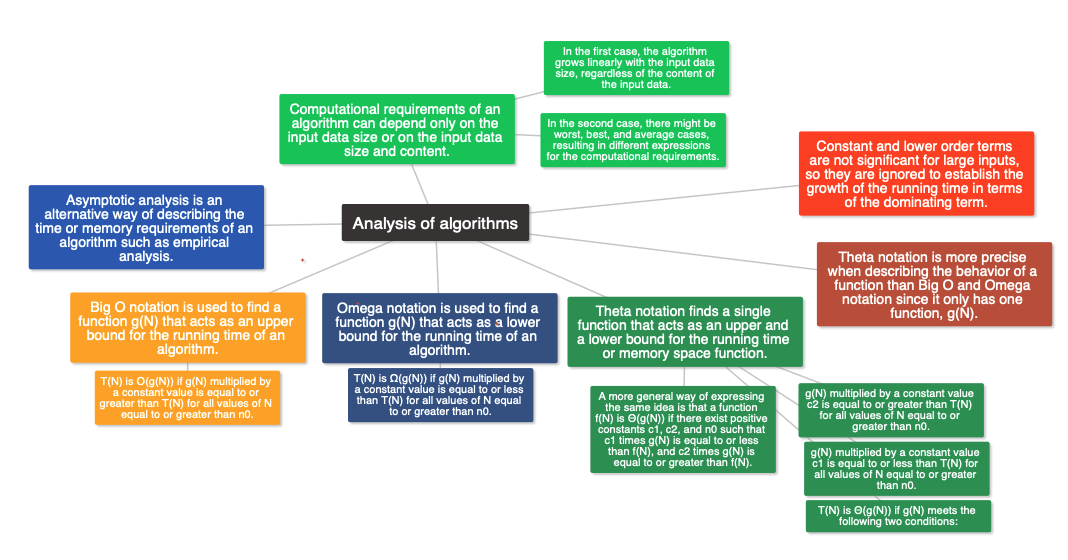
In this lecture, the concept of asymptotic analysis is introduced as an alternative way to describe the time or memory requirements of an algorithm. Asymptotic analysis compares the growth of the running time functions of different algorithms as the input data size approaches infinity. It is based on three notations: Big-O, Omega, and Theta, which were originally devised by mathematicians to describe the behavior of a function when its argument tends to infinity. The use of these notations in analyzing algorithms when the input data is large is called asymptotic analysis.
1.11 Big-O notation
In this lecture, the Big O notation is introduced as a way to describe the time or space requirements of an algorithm. The goal is to find a function g(n) that acts as an upper bound for the algorithm’s resource requirements, T(n). The Big O notation defines a set of functions that can act as an upper bound for T(n). The notation T(n) is O(g(n)) if g(n) is multiplied by a constant value, c, that is equal to or greater than T(n) for all values of n equal to or greater than n0. The lecture provides an example of finding a function g(n) such that T(n) is O(g(n)) for a given T(n) function. The viewer is then asked to find values of c and n0 that make T(n) O(n^3), O(n^4), and O(2^n).
1.12 Omega notation
In this lecture, the Omega notation is introduced, which is similar to the Big O notation but looks for functions that act as a lower bound for the running time of an algorithm. The function T(N) represents the running time of an algorithm, and the aim is to find a function g(N) that acts as a lower bound for T(N). For any function that satisfies this condition, we can say that T(N) is Omega g(N). The formal definition of the Omega notation is provided, and an example is given to demonstrate how to find a lower bound function g(N) that satisfies the condition. Finally, the audience is invited to demonstrate that T(N) is Omega logN and Omega 1 by finding values of c and n0 that make c times g(N) equal to or less than T(N) for all values of N equal to or greater than n0.
1.13 Theta notation
In this lecture, we learned about Theta notation which was created to overcome the limitations of Big O and Omega notations. Theta notation finds a single function that acts as both an upper and lower bound for an algorithm’s running time function or memory space function. We revisited the example from the previous lectures, where t(n) represents the running time of an algorithm, and found that the function g(n) that acts as both an upper and lower bound for t(n) is n^2. We defined Theta notation formally, stating that T(n) is Theta of g(n) if the function g(n) meets two conditions: g(n) multiplied by a constant value c1 is less than or equal to T(n) for all values of n greater than or equal to n0, and g(n) multiplied by a constant value c2 is greater than or equal to T(n) for all values of n greater than or equal to n0. Unlike Big O and Omega notations, which correspond to a set of functions g(n), Theta notation only has one function, g(n), making it more precise when describing the behavior of a function.