2 Recursive algorithms
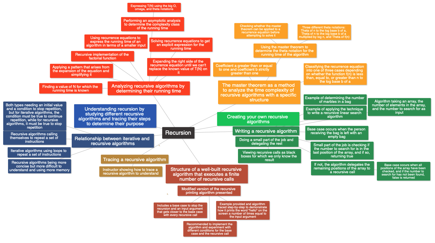
This topic covers recursion in computer science, including understanding, creating, and analyzing recursive algorithms. The structure of a well-built recursive algorithm that executes a finite number of recursive calls is explained, and the importance of tracing recursive algorithms to understand their task is highlighted. The relationship between iterative and recursive algorithms is discussed, and the technique of doing a small part of the job and delegating the rest is explained for writing recursive algorithms. The time complexity of recursive algorithms is analyzed using recurrence equations, and the master theorem is introduced as a method for analyzing the time complexity of recursive algorithms with a specific structure.
2.1 Introduction
This topic is about recursion in computer science, which is the use of an algorithm that calls itself. The topic is divided into three parts. The first part involves understanding recursion by studying different recursive algorithms and tracing their steps to determine their purpose. The second part involves creating your own recursive algorithms, while the third part involves analyzing recursive algorithms by determining their running time. An example of a recursive algorithm is given, which prints “hello” on the screen and then calls itself, resulting in infinite recursion. In the next lecture, a well-constructed recursive algorithm that performs a finite number of recursive calls will be studied.
2.2 The structure of recursive algorithms
This lecture is about the structure of a well-built recursive algorithm that executes a finite number of recursive calls. A modified version of the recursive printing algorithm is presented, which includes a base case to stop the recursion and an input argument that gets closer to the base case with every recursive call. An example is provided, and the algorithm is traced step-by-step to demonstrate how it prints the word “hello” on the screen a number of times equal to the input argument. It is recommended to implement the algorithm and experiment with different conditions for the base case and the recursive call.
2.3 Tracing a recursive algorithm
In this lecture, the instructor shows how to trace a recursive algorithm in order to understand the task performed by the algorithm. They use the example of a function F that takes two integer arguments, a and b, and returns the sum of a and b using recursion. The base case is when b is equal to zero, in which case a is returned. The instructor walks through the process of tracing the algorithm with input arguments of 7 and 3, showing how the recursive calls work and how the value of a is incremented with each call. The final result is 10, the sum of 7 and 3. The key takeaway is that tracing a recursive algorithm can help you understand what task it is performing, even if it is not immediately obvious.
2.4 From iteration to recursion
This lecture explains the relationship between iterative and recursive algorithms. Both types of algorithms repeat a set of instructions, but iterative algorithms use loops to do so, while recursive algorithms call themselves. Both types need an initial value and a condition to stop repetition, but for iterative algorithms, the condition must be true to continue repetition, while for recursive algorithms, it must be true to stop repetition. Recursive algorithms can be more concise, but they are more difficult to understand and use more memory.
2.5 Writing a recursive algorithm - part 1
In this lecture, the instructor explains how to ideate recursive algorithms from scratch. Instead of looking into the details of recursive processing, we should view recursive calls as black boxes for which we only know the result. The instructor uses the example of determining the number of marbles in a bag to illustrate the approach of doing a small part of the job and delegating the rest without caring about the details of how the delegated task is going to be executed. The base case occurs when the person receiving the bag is left with an empty bag. The instructor encourages the viewers to review the recursive algorithms studied so far and identify the small job the algorithm does by itself and the part that gets delegated.
2.6 Writing a recursive algorithm - part 2
In this lecture, the speaker explains how to apply the technique of doing a small part of the job and delegating the rest to write a recursive linear search algorithm. The algorithm takes an array, the number of elements in the array, and the number to search for as input. The small part of the job is checking if the number to search for is in the last position of the array, and if so, returning true. If not, the algorithm delegates the remaining positions of the array to a recursive call. The base case occurs when all positions of the array have been checked, and if the number to search for has not been found, false is returned. The algorithm is then ready for tracing to check its correctness.
2.7 The time complexity of recursive algorithms
In this lecture, we learn how to analyze the time complexity of recursive algorithms. We start with the recursive implementation of the factorial function and define t(n) as the running time of the algorithm for an input size of n. We break down the code into simple operations and use recurrence equations to express the running time of the algorithm in terms of the running time of a smaller input. We end up with an expression for t(n) that is itself recursive and describes the running time of the problem of size n in terms of the running time of a smaller input. This expression is known as a recurrence equation, and we will learn how to solve them in the next lecture.
2.8 Solving recurrence equations
In the previous lecture, we learned about recurrence equations that describe the running time of recursive algorithms. In this lecture, we learn how to solve recurrence equations. To solve a recurrence equation, we need to find a value of N for which the running time is known, and then we expand the right side of the recurrence equation until we can’t replace the known value of T(N) on it. We then apply a pattern that arises from the expansion of the equation, and we simplify it to get an explicit expression for the running time. Once we have an explicit expression for the running time, we perform an asymptotic analysis to determine the complexity class of the running time. We can express T(N) using the big O, omega, and theta notations.
2.9 The master theorem
In this lecture, the master theorem was introduced as a method to analyze the time complexity of recursive algorithms. The master theorem can be applied only if the recurrence equation has a specific structure, where the coefficient a is greater than or equal to one and the coefficient b is strictly greater than one. The theorem classifies the recurrence equation into one of three cases depending on whether the function f(n) is less than, equal to, or greater than n to the log base b of a. After identifying the case, the master theorem can be used to determine the theta notation for the running time of the algorithm. The three cases give three different theta notations, Theta of n to the log base b of a, Theta of n to the log base b of a multiplied by log n, and Theta of f(n). It is important to check whether the master theorem can be applied to a recurrence equation before attempting to solve it.